index_4.html

Metric

We treat several metrics simultaneously. A metric is represented by a symmetric matrix, which entries depend on coordinates. Coordinates are denoted ,,.... The first metric we want to consider is induced by the standard Euclidean scalar product of . Our manifold is with radius r, which we parametrize in polar coordinates below.

$f = r {Cos[x_2] Cos[x_3] Sin[x_1], Cos[x_3] Sin[x_2], Sin[x_3], Cos[x_1] Cos[x_2] Cos[x_3]}$

${r Cos[x_2] Cos[x_3] Sin[x_1], r Cos[x_3] Sin[x_2], r Sin[x_3], r Cos[x_1] Cos[x_2] Cos[x_3]}$

$( {{r^2 Cos[x_2]^2 Cos[x_3]^2, 0, 0}, {0, r^2 Cos[x_3]^2, 0}, {0, 0, r^2}} )$

Parametrizing differently, leads to another matrix g. However, the metric are equivalent.

$f = {x_1, x_2, x_3, (r^2 - x_1^2 - x_2^2 - x_3^2)^(1/2)}$

${x_1, x_2, x_3, (r^2 - x_1^2 - x_2^2 - x_3^2)^(1/2)}$

The computations carried out, are simply the matrix products ..df. In the settings above, df is a 4×3 matrix and =. For instance

$( {{1, 0, 0}, {0, 1, 0}, {0, 0, 1}, {-x_1/(r^2 - x_1^2 - x_2^2 - x_3^2)^(1/2), -x_2/(r^2 - x_1^2 - x_2^2 - x_3^2)^(1/2), -x_3/(r^2 - x_1^2 - x_2^2 - x_3^2)^(1/2)}} )$

Metrics induced by the embedding of the Riemannian manifold are intuitive. Another example is the metric of the geometric torus. Below, we define the domain of the parametrization, and the parametrization itself.

$assum = {0<x_1<2π, 0<x_2<2π, 0<r<R} ;$

$f = {(R + r Cos[x_2]) Cos[x_1], (R + r Cos[x_2]) Sin[x_1], r Sin[x_2]} ;$

$pτ = ParametricPlot3D[Evaluate[f/.(inst = {R→2, r→1})], {x_1, 0, 2 π - 1.5}, {x_2, 0, 2π - 1}] ;$

[Graphics:../HTMLFiles/index_78.gif]

Next, we present three ways to obtain the metric tensor over the particular domain.

$( {{-(R + r Cos[x_2]) Sin[x_1], -r Cos[x_1] Sin[x_2]}, {Cos[x_1] (R + r Cos[x_2]), -r Sin[x_1] Sin[x_2]}, {0, r Cos[x_2]}} )$

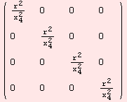
${( {{(R + r Cos[x_2])^2, 0}, {0, r^2}} ), ( {{(R + r Cos[x_2])^2, 0}, {0, r^2}} ), ( {{(R + r Cos[x_2])^2, 0}, {0, r^2}} )}$

Along the metric, we have notions such as the angle between two vectors, and the lengths of vectors, or curves. In general, having defined a volume form on the manifold, we can perform integration on subsets of the manifold. But first, lets continue with metrics of index ≥1. The pseudo sphere of radius r is defined as the points in which annihilate