Computer Graphics


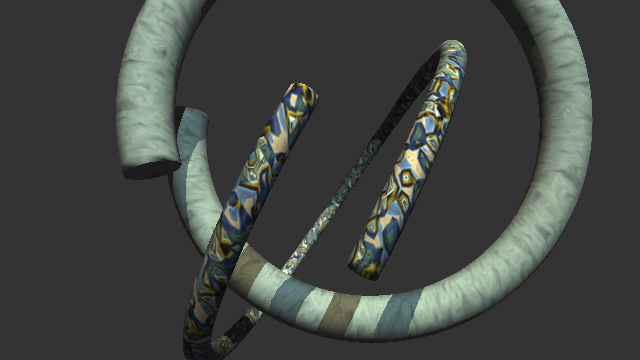
Above, raytraced pics with Deian Tabakov. Unfortunately, the code is lost. I made a new raytracer. Even more ancient: Fractals in PowerBASIC

Interactive World Simulation
Wave Particles et cetera
Color3D
Jaya · 3D Modeling and Deformation
Texture Advection for Fluid Flow
Single Image Stereogram
Edge-Aware Filtering
The woods are lovely, dark, and deep,
But I have promises to keep,
And miles to go before I sleep,
And miles to go before I sleep.
Robert Frost

Texture Advection for Fluid Flow


Resulting animation from flame pattern

The following work is inspired by the PhD thesis "Models of Animated Rivers for the Interactive Exploration of Landscapes" of Qizhi Yu.

When they tell you not to panic,
that's when you run!
John Cusack

An overview: From a map of shores, we construct a static flow in the space between the shores. This space is called river. Triangular patches textured with lava or water patterns are sampled in the river. The vertices of the patches undergo the flow individually. Over time the patches become vastly distorted and fade out. New undistorted patches are introduced in their place.

To derive a static flow for a given river network, we define a potential function that is constant on each single shore. The total flow between to shores will match the difference in the potential function evaluated on the two corresponding shores.


To derive the flow, we interpolate the potential function in the river using Shepard's formula with coefficient p=2. The formula requires a notion of (minimal) distance for a given point in the river and a shore. We obtain these distance functions by computing shortest paths from each shore to all points in the river. The paths are restricted to the river.


We denote by the interpolation of the potential function in the domain of the river. The point lies in the river. The flow is the vector field defined by the numeric partial differentials . In general, the function is not smooth, thus the partial differentials might be discontinous causing the flow to change direction abruptly. However, is divergence free to emulate incompressable fluid.


To create the visual effect of the flow, we equip planar triangular patches with a random piece of the texture. The texture of the patch fades out into transparency beyond a certain radius r around the center. Beyond a radius of 2r, the patch is transparent.


Poisson disc sampling

The verticies of a patch undergo the flow velocity individually. In general, the patch deforms. Since a patch starts consisting of equilateral triangles, we can measure the deformation simply by evaluating the edge lengths of the deformed patch.


To balance the visual appearance and computational load, we ensure that these patches remain separated by at least radius r, and yet are tighly packed. Our sampling algorithm follows the method Fast Poisson disk sampling in arbitrary dimensions by Robert Bridson.


textural flow of water, fire, foam, hardwood flooring

The evolution of such a poisson disk sampling is shown in the animation aside. In case two patches have moved closer than 2r, the more deformed fades out (marked by a red dot) while the less deformed remains a Poisson disc sample (green). The removal of patches might leave a gap that is big enough to contain a new patch. The sampling algorithm detects these gaps and locates a new, undeformed patch at that point. The patch is made to slowly fade in to the environment.

Texture Advection for Fluid Flow (Demo with source in C++) textureflow.zip 1.4 MB

Correct blending requires that patches are drawn in the order that they were introduced. To yield appealing results, the texture spectrum and patch radius need to be in tune.

L'avenir, tu n'as point à le prévoir mais à le permettre.
Antoine de Saint-Exupéry

Single Image Stereogram


scene

depth

stereogram (click to enlarge)

The algorithm is adapted from Real-Time Stereograms of the book 'GPU Gems'.

function bmp=stereogram(depth)
% creates greyscale single-image-stereogram of depth field
%  depth     (n,m)-matrix
% which has values in the interval [0,1]
% please scale depth so that an entry with value
%  0 is farthest
%  1 is closest
% the algorithm works best if
%  m ranges between 480 and 1280
    
ofs=80;
sca=16;

bmp=repmat(uint8(rand(size(depth)+[0 ofs])*255),[1 1 3]);
for cy=1:size(depth,1)
  acc=0;
  for cx=1:size(depth,2)        
    inc=depth(cy,cx)*sca+acc;
    res=floor(inc);
    acc=inc-res;
    bmp(cy,ofs+cx,:)=bmp(cy,cx+res,:);
  end
end    
bmp(:,1:ofs,:)=[];
imshow(bmp)

The use of random noise texture is suitable for animations.


If you have a problem,
and you can't solve it alone,
evoke it.
African proverb

Edge-Aware Filtering


face

flower

puzzle

castle

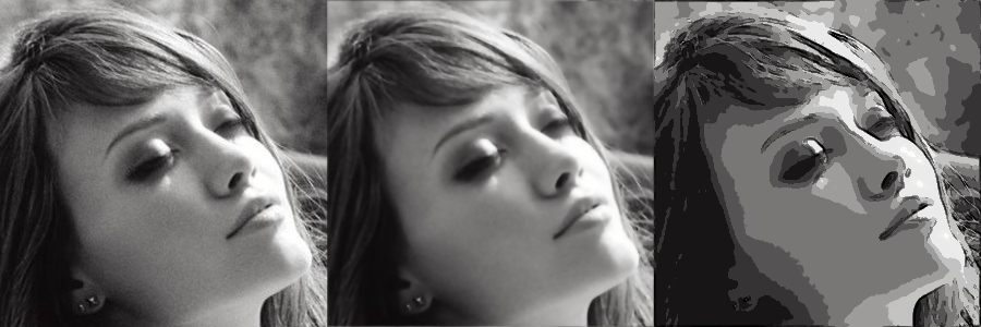
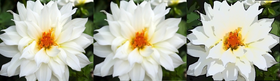
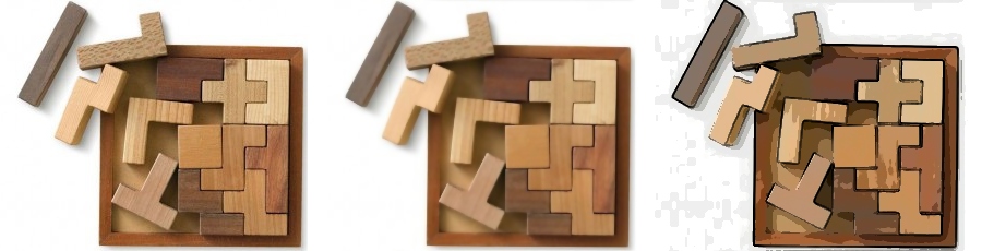
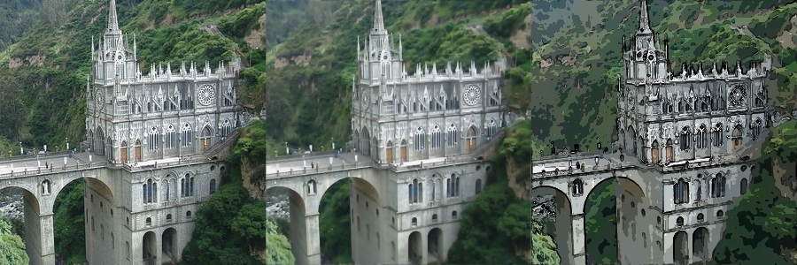
Eduardo Gastal and Manuel Oliveira have introduced a simple and efficient algorithm to carry out edge-aware image transformations, for instance edge-preserving smoothing. Their method Domain Transform for Edge-Aware Image and Video Processing was published at Siggraph 2011.

Douglas R. Lanman shares source code on Bilateral Filtering. The package also contains a nice cartoon renderer. I have replaced his implementation of the edge-preserving filter with the new, faster algorithm, to speed up the cartoon renderering.

Edge-Aware Filtering (Matlab) * edgeaware.zip 270 kB
cartoon.m by Douglas R. Lanman, colorspace.m by Pascal Getreuer.

Below is the 40 lines listing of my implementation in Matlab. The emphasis is on simplicity and compactness:

function img=edgeawared(img) % img has double values between 0 and 1

for wid=[3 1]; % support of filter
  for c1=1:size(img,1)
    dom=ji1domain(img(c1,:,:));
    for c3=1:size(img,3)
      img(c1,:,c3)=ji1edgeaware(wid,img(c1,:,c3),dom);
    end
  end
  for c1=1:size(img,2)   
    dom=ji1domain(img(:,c1,:));
    for c3=1:size(img,3)
      img(:,c1,c3)=ji1edgeaware(wid,img(:,c1,c3)',dom)';
    end
  end
end  

function dom=ji1domain(sig)
  sz=size(sig);
  sz(find(sz==1))=[]; 
  sig=reshape(sig,sz)';
  dom=cumsum(1+sum(abs([zeros(sz(2),1) diff(sig,1,2)]),1));

function res=ji1edgeaware(w,sig,dom)
  if nargin==2
    dom=cumsum(1+[0 abs(diff(sig))]);
  end
  dom(end)=ceil(dom(end)); % small error happens here
  smp=1:dom(end);
  itr=interp1(dom,sig,smp);  
  res=interp1(smp,ji1filter(w,itr),dom);

function res=ji1filter(w,sig)
  w=2*w+1;
  x=linspace(-2,2,w);        
  fil=sqrt(1/pi)*exp(-x.*x); 
  fil=fil/sum(fil);          
  num=numel(sig);
  f_sig=fft(sig);
  f_fil=fft(fil,num);  
  res=ifft(f_sig.*f_fil);
  res=real(res);    
  res=res([(w+1)/2:end 1:(w-1)/2]);

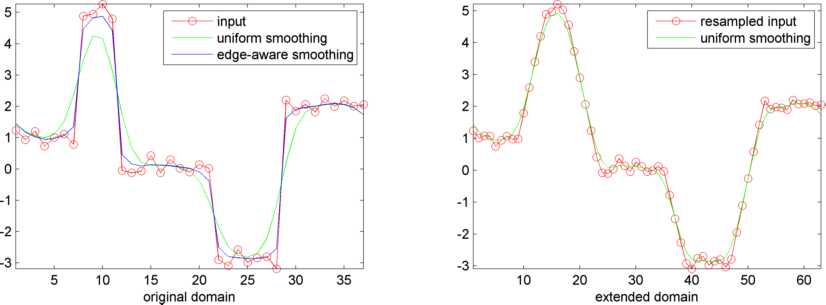
The figure below illustrates how the algorithm operates on a 1-dimensional domain. The signal is warped onto a streched domain and resampled uniformly. This allows to apply a standard gaussion smoothing filter. Inverting the warp and resampling over the original domain yields the smoothed signal with edges preserved.

The extraordinary is in what we do,
not who we are.
Lara Croft