Vision Payload with Radiation Tolerant CMOS Sensor

radiation tolerant CMOS sensor

pixel 0.0065 mm

The vision payload was developped for a nano satellite at Nanyang Technical University/Singapore. The purpose of the payload is

• to take greyscale images of the Earth at altitudes of around 650 km, and
• to test the suitability and robustness of the self-designed CMOS chip.

The optical system is designed so that at a distance of 650 km, one pixel width corresponds to 21 m on ground. The image resolution is 768 x 512.

The payload consists of four blocks of hardware:

• PC/104 single-board-computer "Cool SpaceRunner-LX800" by Lippert Embedded Computers GmbH for image processing and compression
• Opal Kelly XEM3005 with the Spartan-3E FPGA XC3S1200E for sensor control and data acquisition
• printed circuit board equipped with a CMOS sensor designed at NTU
• optical system: three lenses, steel apperture, and shielding

The CMOS image sensor for satellite remote sensing application was designed by researchers on semi-conductors at Nanyang Technical University. See their chip gallery. I quote their description of the sensor:

"Radiation-tolerant image sensor for space applications (Version 2): [...] In particular, the CMOS image sensor will address a number of challenges such as space radiation wide range of operating temperature as well as limited exposure time. [...] The sensor was designed for use in space and avionics systems. A number of techniques were employed to address space-radiation induced effects such as leakage current, SEU and Vt shift. Other features include: dynamic gain/exposure control, temperature compensation. [...]"

Following the modeling phase, the chip was manufactured by TSMC, the Taiwan Semiconductor Manufacturing Company in 2011. More information on the website of Chen Shoushun.

Analysis of Three Lens Optical System with CMOS sensor	vision_payload.nb	90 kB
Analysis of Three Lens Optical System with CMOS sensor	vision_payload.pdf	220 kB

The array of the sensor has 768 x 512 pixels. Each pixel encodes an illumination intensity on a 12-bit grayscale, i.e. the value ranges from 0 to 4095. However, the noise in each pixel is approximately normal distributed with a standard-deviation of ±14.5 on the greyscale, which is equivalent to 4 bit. Consequently, the effective resolution of intensity is reduced to 8-bit due to noise.

To achieve high read-out speeds, the CMOS sensor array is connected to and controlled by the Spartan-3E FPGA XC3S1200E. The FPGA itself is mounted on a 3rd-party development-kit Opal Kelly XEM3005 (ver. 20081010). The firmware of the FPGA is developped by the chip designers at NTU, and provided in binary format.

If you are neutral in situations of injustice,
you have chosen the side of the oppressor.
Desmond Tutu

Optical system

light enters the camera from the bottom

The lens system consists of three lenses with the following curvatures:

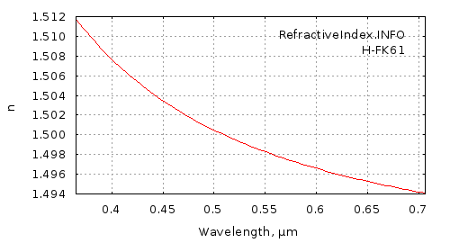
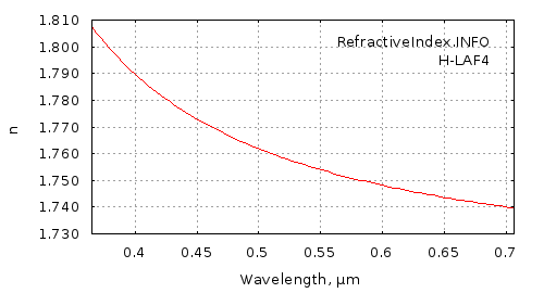
Lens 1 and 2 are made of Fluor Crown H-LAF4. Lens 3 is made of Lanthanum Flint H-LAF4. The refractive index depends on the wavelength of light. The following graphs are from refractiveindex.info:

• 
  refractive index of Fluor Crown H-LAF4
• 
  refractive index of Lanthanum Flint H-LAF4

Refraction causes white light to appear as rainbow color. Wikipedia has a good illustration for chromatic aberration. The selection of Lens 3 is to mitigate this optical effect caused by Lens 1 and 2.

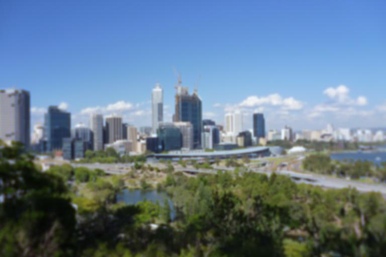
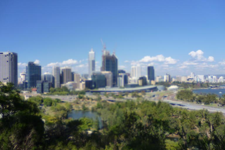
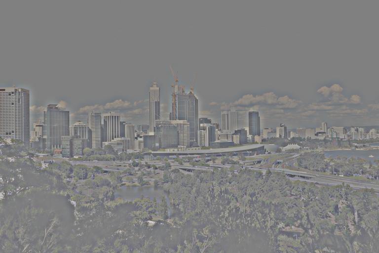
The field of view is 1.43 degree along the width of the array and 0.95 degree along the height of the array. These are some of the first pictures taken with the real lens:

In a wild barely inhabited landscape
any soldier at all is an eyesore.
H. W. Tilman

Raytracing results

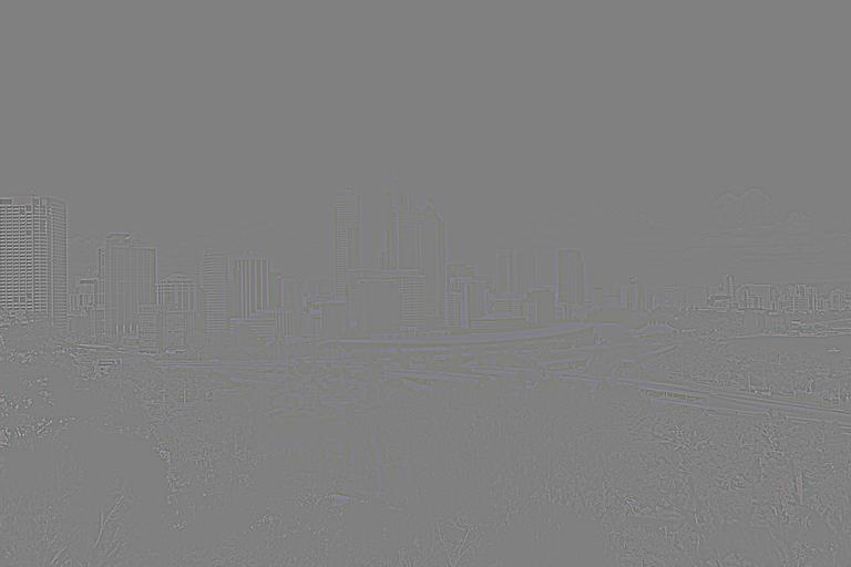
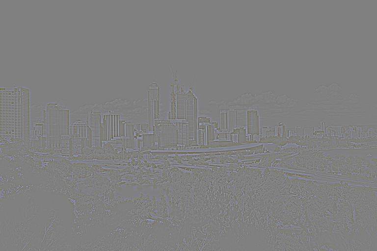
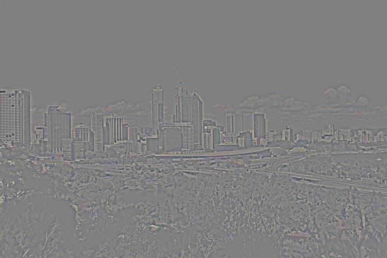
We investigate the effect of an unintended offset between the lens and the CMOS array. The images show the blur introduced due to a misalignment of the following magnitudes: 0, +0.1, -0.1, 0.2, and 0.5 mm. The effect depends on the wavelength as well as the angle. That means, that even if the image is razor-sharp in the center, the edges exhibit blurriness.

• 
  original
• 
  0.0 mm
• 
  0.1 mm
• 
  -0.1 mm
• 
  0.2 mm
• 
  0.5 mm
• 
  0.0 mm (diff)
• 
  0.1 mm (diff)
• 
  -0.1 mm (diff)
• 
  0.2 mm (diff)
• 
  0.5 mm (diff)

The raytracing in our simulation is implemented in 2d. For more accurate results, for instance to reverse engineer a blurred image, a simulation in 3d is desirable.

To see a world in a grain of sand,
and a heaven in a wild flower.
Hold infinity in the palm of your hand,
and eternity in an hour.
William Blake

Digital image acquisition

T3Z3510CS-IR

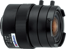
For indoor testing and short-range outdoors, we use the Computar T3Z3510CS-IR lens that has the following optical characteristics:

The lens weights 63g. The diameter is 41.6mm, the height is 48.8mm. The lens is attached to the PCB via CS-mount, and operates in temperatures between -20 to 50 deg C.

The experiments and calibrations below are performed with the NTU Radiation-Tolerant CMOS Image Sensor Chip-3 PCB-2 and the T3Z3510CS-IR lens.

black standard deviation

black standard deviation

Main clock and exposure clock

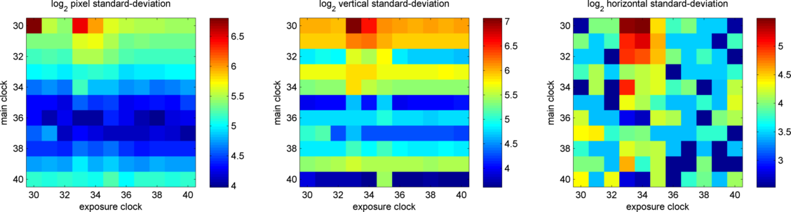
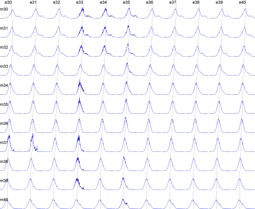
The main clock provides the timer to the FPGA. The function of the exposure clock is not know to us at this point. Both clock register values range from 30 to 40. However, both clock values determine the quality of the image.

We perform the following experiment: The lens is covered with a lid to prevent the exposure of the CMOS sensor to light. Then, we sweep through all possible pairs of clock values, taking 20 exposures for each tuple. We average the images for each clock value tuple and form the distribution of grayscale values, as well as correlation of adjacent pixels.

The graphics to the side show the results. The noise distribution varies significantly with the choice of clock values.

• to minimize the pixel noise variance, the main clock register should range between 35 - 38.
• to maximize the correlation of the vertical adjacent pixels, the main clock register should be set to 35, 37, or 40.
• to maximize the correlation of the horizontal adjacent pixels, the main clock and exposre clock values can be selected from the list:
  (35,32), (36,38), (37, 40), (38, 39), (39, 37), ..., (40, 36).

For our final algorithm, we combine these rules of thumb. The list of clock value register tuples that the exposure mechanism chooses randomly from is

(40, 39), (39, 34), (39, 32), (37, 40), (37, 39), (37, 38), (37, 32),
(36, 40), (36, 39), (36, 38), (36, 37), (36, 36), (35, 32).

fixed pixel bias

Fixed pixel bias

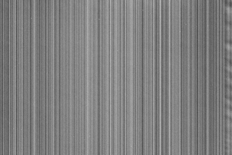
Fixed pixel bias denotes the average intensity perceived by the pixel location when the exposure occurs in total darkness. In total darkness, all pixels should ideally read out identical values (since the light intensity is the same for all pixels). However, due to irregularities in manufacturing, each pixel and in particular each column has it's own characteristic bias. The bias can be established by taking a great number of images in total darkness and averaging the captured intensities.

The pixel bias does not noteably change over time and is therefore called fixed bias. Moveover, the bias is added to the pixel regardless of intensity. That means, once the pixel bias is established, it can be substracted from a regular exposure to significantly improve imaging quality.

Here is pseudo MATLAB code to finalize the fixed pixel bias:

  % avg is the average of the sum of all exposures in total darkness. avg is a [512 768] matrix.
  fpn=avg-repmat(mean(avg,2),[1 768]); % subtracting the mean for each line gives the best result

black level for ref and exp

Reference voltage of the analog-to-digital conversion

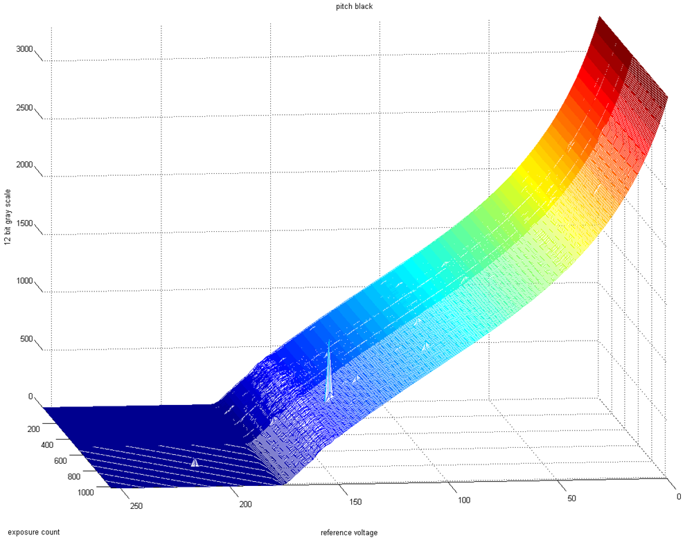
The charge collected by a pixel is ultimately converted to a voltage by an analog-to-digital converter (ADC). The output of the ADC is a value between 0 and 4095, corresponding to a 12-bit range.

The ADC requires a reference voltage to compensate a constant bias in the amplification process. The reference voltage determines to what output value the pixels are mapped, that are not exposed to light. The figure on the side shows that this mapping is independent of exposure time.

The reference voltage is set by a byte value 0, 1, ..., 255 in software. Altering the reference voltage simply causes a linear shift of the grayscale values. Thus the reference voltage is optimal, when black pixels are mapped to a grayscale value slightly above 0. That way, the full 12-bit range is available for the mapping of brighter pixels.

The byte value that determines the reference voltage is not a variable. In our experience, the byte value does not require changing. We fix the value to 170 (see figure).

exposure time vs mean grayscale

mean grayscale vs compressed image size

Exposure time

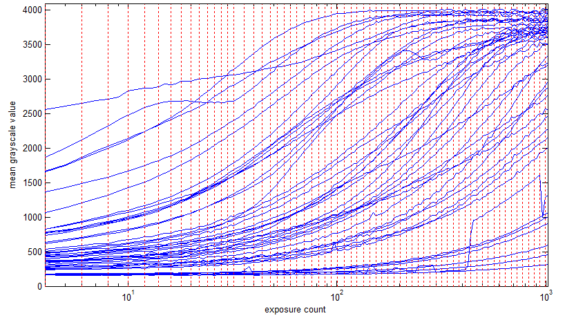
Exposure time has the great impact on image quality. Exposure time affects the contrast of the image. Typically, an image with good contracts has a spread distributation of grayscale values.

• if the exposure time is too small, the image exhibits mostly dark pixels
• if the exposure time is too large, the image exhibits mostly white pixels

The video shows pictures taken outdoors in different lighting conditions. For each motive, we take several exposures with different exposure times each. The correlation of exposure time and mean grayscale value is shown on a logarithmic scale in the figure to the right. Each blue line corresponds to a separate motive. The lines are similar in shape, and only vary by an offset along the x-axis.

In order to obtain an image with good contrast, the exposure time needs to be chosen just right. The exposure time does not relate to average intensity, i.e. mean grayscale, in a linear fashion. Our experiments suggest, that for each scene, there is a region on the exposure time logarithmic scale, where the average intensity increases linearly. Once the average intensity approaches a limit, it does not increase significantly anymore.

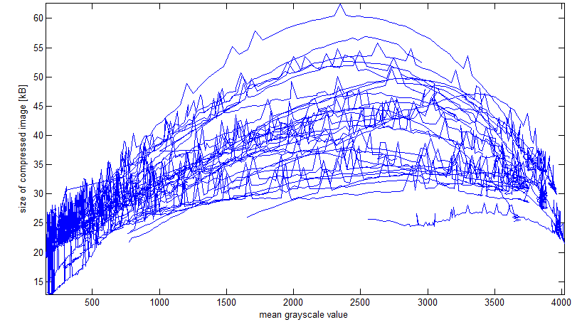
Above, we mentioned that the average intensity should ideally be medium gray. In order to back that claim, we evaluate the file sizes of the images in their compressed format. A low file size means, little information remains in the image, when compared to an image of the same scene with a larger file size. Our experiments suggest that the maximum file size is not obtained at the exact medium intensity, i.e. 50% grayscale, but above that value namely around 60% grayscale value.

For a static scene, one can design an iteration that finds the exposure time that results in a mean grayscale value of say 50%, i.e. 2048. The iteration could take into account the characteristic exposure time to mean grayscale curve. However in space, the camera view is dynamic: The narrow field of view of 1-2 degrees, and the rotation of the satellite cause that the scene changes rapidly. That means for two successive exposures the lighting condition are subject to change. In order to optimize the exposure time, we do not want to rely on an iterative method.

We define a list of 10 exposure times, that are evenly spaced on a logarithmic scale. To acquire a single image, we take 10 pictures each with a unique exposure time from the list. Among the 10 images taken, we select the one that has the mean grayscale value closest to say 50%, i.e. 2048. Another detail: The list is randomly shuffled before each image acquisition.

Curiosity is an everlasting flame that burns in everyone's mind.
It makes me get out of bed in the morning and wonder
what surprises life will throw at me that day.
Curiosity is such a powerful force.
Without it, we wouldn't be who we are today.
Curiosity is the passion that drives us through our everyday lives.
We have become explorers and scientists with our need to ask questions and to wonder.
Clara Ma

Data compilation and transfer

The resulting image is 12-bit grayscale image with 393216 pixels. Uncompressed, the data takes up 589824 bytes, almost 600 kB. The steps in the image processing and compression are guided by the following observations:

• the noise amplitude is about 4 bits (according to the experiment described above)
• the color values in the very dark and very bright region might not be used due to particular lighting conditions
• the raytracing simulation shows that a minimum amount of blurriness is to be expected
• the downlink rate via radio transmission is around 200 B/sec

The image processing and compression consist of the following steps:

We first cut off the unused regions of the 12-bit grayscale palette and strech the interior region to the full grayscale. Then, the 4 least-significant-bits of each 12-bit color value are dropped. In order to maximize the chances of reverse engineering any blurriness, we favor loss-less PNG-compression over the lossy JPG-compression. Since file size is also a concern, we perform the following comparsion: If the PNG-compressed image is less than 200 kB, we select the PNG-file for downlink, else we take the JPG-file.

The thumbnail is a derived from the uncompressed 8-bit image. To avoid aliasing, we subsample the image in an iteration of scaling operations, each reducing the sides by a factor of 1/sqrt(2)=0.707107. The iteration stops when the JPG-compressed version of the thumbnail falls below 4 kB. As render parameters for the downscaling we make use of the bilinear interpolation and anti-aliasing options:

private static BufferedImage resize(BufferedImage myBufferedImage, double factor) {
  int width = (int) Math.round(myBufferedImage.getWidth() * factor);
  int height = (int) Math.round(myBufferedImage.getHeight() * factor);
  BufferedImage resizedImage = new BufferedImage(width, height, image_type);
  Graphics2D myGraphics2D = resizedImage.createGraphics();
  myGraphics2D.setComposite(AlphaComposite.Src); // to prevent transparency
  myGraphics2D.setRenderingHint(RenderingHints.KEY_INTERPOLATION, RenderingHints.VALUE_INTERPOLATION_BILINEAR);
  myGraphics2D.setRenderingHint(RenderingHints.KEY_RENDERING, RenderingHints.VALUE_RENDER_QUALITY);
  myGraphics2D.setRenderingHint(RenderingHints.KEY_ANTIALIASING, RenderingHints.VALUE_ANTIALIAS_ON);
  myGraphics2D.drawImage(myBufferedImage, 0, 0, width, height, null);
  myGraphics2D.dispose();
  return resizedImage;
}

The output of each image acquisition are three items:

• thumbnail JPG file less than 4 kB
• full resolution JPG file less than 200 kB
• 32x32 pixel subimage with 12-bit grayscale resolution from central image region for the analysis of raw data. also, two temperature values from the SBC chip and board in 1 deg accuracy.

Unfortunately, Java does not allow the programmer to choose the compression parameter. But Java can display semi-complete JPG files, which is suitable when receiving the an images through radio connection.

We also experimented with the PNG format. But photos of natural scenes are noisy and grainy, and result in large PNG files even if displaying not particularly interesting content. Another reason for dismissing PNG was that no preview of semi-complete PNG files was possible in Java.

The data is split into a sequence of frames of 220 bytes. A 16-bit checksum ensured the consistency of each frame. The frames are forwarded to microcontrollers via serial port and system management bus (SMBus).

Chromosomal crossover is like an elephant repellent.
You know it's working because you don't see any elephants.
Matt Ridley

Images from space at 650 km altitude

happy about first images from space

The nano-satellite was launched on the 2014-06-30. The first image acquisition took place on the 2014-07-02 with no particular target in mind, but simply to check if the computer systems were working. The image acquisition took the typical duration which was a good sign. Three thumbnail images of around 1.5kB each were downloaded one day later, on the evening of 2014-07-03. The results confirmed that the camera worked. More pictures were taken and downlinked later.

You have not converted a man
because you have silenced him.
John Morley