Numerics provides approximate answers to real world problems.
|
|
|
|
|
|
|
|
|
|
There never will be any good, general methods for
solving systems of more than one nonlinear equation.
Press, Teukolsky, Vetterling, Flannery
We present a computation to yield the transformation that matches best two given sets of landmarks on a linearized homogeneous manifold. The method allows to restrict the set of feasible transformations in a way that is most relevant in practical applications. If the homogeneous manifold is a vector space, the transformation is optimal in the limit.
Time is nature's way of keeping
everything from happening at once.
Allen Stewart Königsberg
| Tracking on Homogeneous Manifolds |
|
180 kB |
| Examples and illustrations (Mathematica 5.2) * |
|
35 kB |
Our computation is an alternative to the conventional algorithms in tracking (that might utilize quaternions, or Euler-angles). Our method minimizes the sum of squared errors between the pairs of landmarks in the match. The number of variables is precisely the dimensions of the mobility of the robot. To solve the non-linear equations, Newtons iteration works well.
In the paper, Meshless Deformations Based on Shape Matching by M. Mueller, B. Heidelberger, M. Teschner, M. Gross an optimal rotation is found via the polar decomposition of a matrix. This motivated me to make a tracking algorithm using the Campbell-Baker-Hausdorff series in the more general context of homogeneous manifolds.
If everything seems under control,
you're just not going fast enough.
Mario Andretti
Given a set of points, we find the center and radius of a sphere that fits the points well. The method is extracted from code of Izhak Bucher.
In
 dimensional Euclidean space, points
 on a sphere with center
 and radius
 are characterized by

Equivalently,
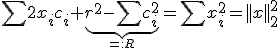
where the summations are over the coordinates
 .
Now, we are given a set of
.
Now, we are given a set of
 points

To obtain the center of the fitting sphere
 ,
we solve the following system of linear equations in the least square sense
,
we solve the following system of linear equations in the least square sense
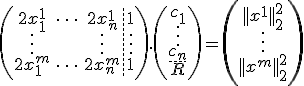
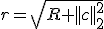
Then, the radius of the sphere is
If the matrix above does not have maximum rank, we define
 .
.
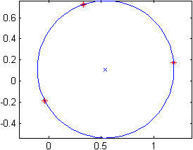
As desired, the radius of the sphere is invariant under affine transformation of the points, while the center of the sphere undergoes the same affine transformation. The method is implemented by the following function in Matlab, download.
function [c,r]=spherefit(X,draw)                % code by jph
%syntax:   [C,R]=SPHEREFIT(X,DRAW)
% X is of size [m n] and contains m points of dimension n.
% C is the center, and R is the radius of the fitting sphere.
% If DRAW is specified and n==2, the result is plotted.
%example:  [c,r]=spherefit(randn(7,2),1)

n=size(X,2);
A=[2*X ones(size(X,1),1)];

if rank(A)<n+1
  c=[];
  r=Inf;
  return;
end

a=A\sum(X.*X,2);
c=a(1:end-1);
r=sqrt(a(end)+c'*c);

if nargin>1&&n==2
  plot(X(:,1),X(:,2),'r*');
  hold on; axis equal;
  plot(c(1),c(2),'bx');
  t=linspace(0,2*pi);
  plot(r*cos(t)+c(1),r*sin(t)+c(2),'b');
  hold off;
end
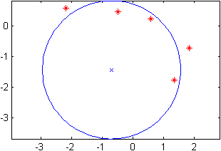
The following example corresponds to the two dimensional scenario.
To infinity and beyond.
Buzz Lightyear
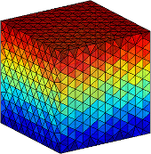
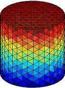
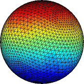
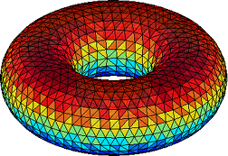
We release Matlab code to create triangulations of four basic shapes in three dimensions: cube, cylinder, sphere, torus. The functions are
[T,X,Y,Z]=tricube(n);
[T,X,Y,Z]=tricylinder(n);
[T,X,Y,Z]=trisphere(n);
[T,X,Y,Z]=tritorus(R/r,n);
The parameter n controls the granularity. The generation of the torus requires an additional parameter: the ratio of the big and small radius R/r. To visualize the outputs simply use the Matlab command
trimesh(T,X,Y,Z);
| Triangulations of elemental shapes in Matlab * |
|
50 kB |
Nullius in verba