Differential Geometry

Humboldt-University zu Berlin

Campus Adlershof

At the Humboldt-University zu Berlin, I specialized in differential geometry, in particular semi-Riemannian geometry, and Lie theory. The concepts are used in physics to fomulate:

• the motion of rigid bodies, as well as
• general relativity theory.

In 2006, I submitted my diploma thesis on Lorentzian Ricci-flat homogeneous manifolds.

On Lorentzian Ricci-flat Homogeneous Manifolds

Ricci-flat Invariant Geometry in Four Dimensions

Raytracing Special Relativity

Hoffnung ist nicht die Überzeugung, dass etwas gut ausgeht,
sondern die Gewissheit, dass etwas Sinn hat, egal wie es ausgeht.
Václav Havel

Weighted averages and barycentric coordinates in non-linear spaces

My work at ETH Zürich/Switzerland in 2017–2019 in robotics has inspired the following results:

Smoothing using Geodesic Averages

Inverse Distance Coordinates for Scattered Sets of Points

Biinvariant Generalized Barycentric Coordinates on Lie Groups

Biinvariant Distance Vectors

The articles related to weighted averages, subdivision, smoothing and biinvariant barycentric coordinates are lined up below for quick access:

• 
  article 412kB, video
• 
  article 1.7MB, video
• 
  article 1.2MB
• 
  article 2.5MB, video
• 
  article 2.3MB

Having eyes, but not seeing beauty;
having ears, but not hearing music;
having minds, but not perceiving truth;
having hearts that are never moved and therefore never set on fire.
These are the things to fear, said the headmaster.
from Totto-Chan

Miscellaneous

The posts below are transcriptions of methods developed by other researchers:

Biharmonic Distance

Spin Transformations

Tensor fields are the essence of differential geometry. Relevant computations, such as the determination of the Riemannian curvature, usually are not doable by hand. All this is covered in our differential geometry package for Mathematica 5.2. We also provide operations related to Lie algebras and Lie groups.

Differential Geometry with Mathematica
Latest version of the (DG)kernel notebook
Documentation
Tensors
Manifolds
Lie-algebras
Lie-groups

The beauty of Nature lies in detail; the message in generality.
Optimal appreciation demands both and I know no better tactic than
the illustration of exciting principles by well-chosen particulars.
Stephen Jay Gould

On Lorentzian Ricci-Flat Homogeneous Manifolds

two parametrizations of moduli spaces of 4-dimensional Lorentzian homogeneous
triples with isotropy dim h=1, and curvature Ric=0

The chapter "Introduction" from my thesis:

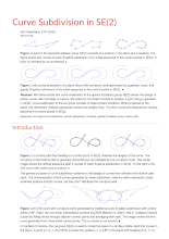
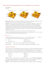
A homogeneous space is the coset manifold G/H, where G is a Lie group, and H is a closed Lie subgroup of G. The canonic mappings related to a homogeneous space are the projection, and the left-action. The differential of the left-action extends tensors of special form to invariant tensor fields on the manifold G/H. For instance, an invariant metric on G/H originates from a single scalar product B. A homogeneous triple associated to the homogeneous space G/H with invariant metric is (g,h,B), where g is the Lie algebra of G, h<g is the subalgebra induced by the subgroup H, and B is the scalar product on a vector space complement m with g=h+m induced by the metric.

For a homogeneous space with invariant metric, geometric notions such as the Levi-Civita connection, and the curvature can be derived at a single point of G/H in terms of the homogeneous triple. The curvature tensor obtained this way translates to the invariant curvature tensor field on the semi-Riemannian manifold G/H. Locally, the homogeneous triple uniquely determines the corresponding semi-Riemannian homogeneous space. In the thesis, we are interested in homogeneous triples that relate to homogeneous spaces with the following geometric properties:

• The invariant metric is Lorentzian.
• The Riemannian curvature is non-zero.
• The space is Ricci-flat.

Metrics of index 1 are the core in relativity theory. From the geometric viewpoint, Riemannian-flat homogeneous spaces are not particularly interesting. A Ricci-flat homogeneous space is naturally an Einstein manifold.

On Lorentzian Ricci-Flat Homogeneous Manifolds (Thesis) *	lorentzian_ricci...	630 kB
Details to Example 3.7	thes_exm37	link

* submitted on the 30th Sep 2006 as Diplomarbeit

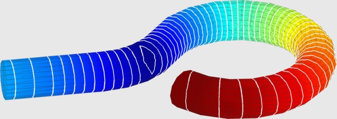
The major contributions are summarized on the last page of the thesis. The picture above visualizes two parametrizations of moduli spaces of 4-dimensional Lorentzian homogeneous triples with isotropy dim h=1, and curvature Ric=0.

And the end of all our exploring
will be to arrive where we started
and know the place for the first time.
Thomas Stearns Eliot

Subsequently, two research papers have cited the thesis:

If not now, then when?
If not me, then who?

Biharmonic Distance

Hook

Sphere

Beethoven bust

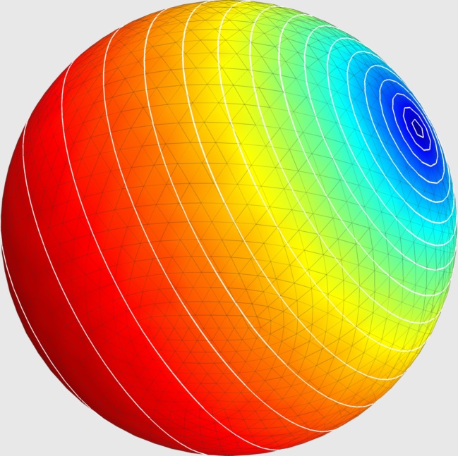
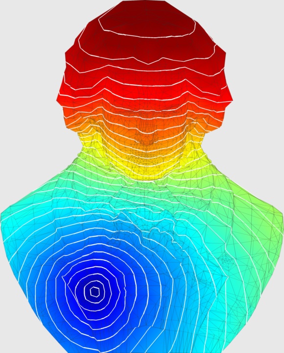
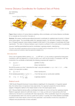
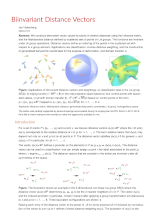
Yaron Lipman, Raif M. Rustamov, and Thomas A. Funkhouser introduced Biharmonic Distance at Siggraph 2011. Biharmonic distance is a construction of a metric on a continous or discrete (triangulated) surface. The resulting metric d(x,y), i.e. a notion of distance between points x and y, has very desirable properties. I quote from the paper:

• smooth with respect to perturbations of x and y, with no singularities except derivative discontinuity at x
• approximately geodesic when y is near x
• reflects overall shape of the surface when y is far from x
• does not change with isometric transformations of the surface
• does not change significantly with the addition of noise or changes to topology
• compute times between all pairs of points in common meshes take at most a few minutes
• parameter-free

Biharmonic Distance (Matlab) *

biharmonic.zip

170 kB

* for a demo run biharmonicdemo.m in Matlab.

My implementation that is listed below works well for triangulated meshes with less than 3k vertices.

function dB=biharmonic(T,V)
% input: T (3xN) and V (3xM) so that
%  trimesh(T',V(1,:),V(2,:),V(3,:))
%  plots the triangular mesh
% output: dB (MxM) matrix where dB(i,j)
%  is distance between vertex i and j

nT=size(T,2);
nV=size(V,2);

AT=zeros(nT,1);
for c1=1:nT
  pnt=V(:,T(:,c1));
  AT(c1)=norm(cross(pnt(:,2)-pnt(:,1),pnt(:,3)-pnt(:,1)));
end

AV=zeros(nV,1);
ind={};
for c1=1:nT
  c3=T(:,c1);
  AV(c3)=AV(c3)+AT(c1);
  for c2=[c3 c3([2 3 1]) c3([3 1 2])]
    i=c2(1);
    j=c2(2);
    k=c2(3);
    v1=V(:,i)-V(:,k);
    v2=V(:,j)-V(:,k);
    fac=norm(v1)*norm(v2);
    if fac<eps
      fprintf('triangle %i is degenerate\n',c1)
    else
      val=cot( acos( dot(v1,v2) / fac ) );
      ind{end+1,1}=[
        i i  val
        i j -val
        j i -val
        j j  val
      ];
    end
  end
end
ind=cell2mat(ind);
Lc=sparse(ind(:,1),ind(:,2),ind(:,3),nV,nV);

gd=pinv(full(Lc*spdiags(6./AV,0,nV,nV)*Lc));
dia=diag(gd);
dB=zeros(nV);
for i=1:nV
  dB(:,i)=sqrt(gd(i,i)+dia-2*gd(:,i));
end

The command pinv is chosen for simplicity and stability, because the Matlab command svds for sparse matrices does not neccessarily converge. Section 3.3 Practical Computation in the paper describes how to solve a series of systems of linear equations to yield the exact metric in a more efficient computation.

Alec Jacobson in his 2013 PhD Thesis "Algorithms and Interfaces for Real-Time Deformation of 2D and 3D Shapes" explains how the sophisticated notion of distance helps to model weight functions. The weight functions interpolate between linear transformations that represent deformations.

I suggested that we might compare earthquakes in terms
of the measured amplitudes recorded at these stations,
with an appropriate correction for distance.
Charles Francis Richter

Spin Transformations

input 1

output 1

input 2

output 2

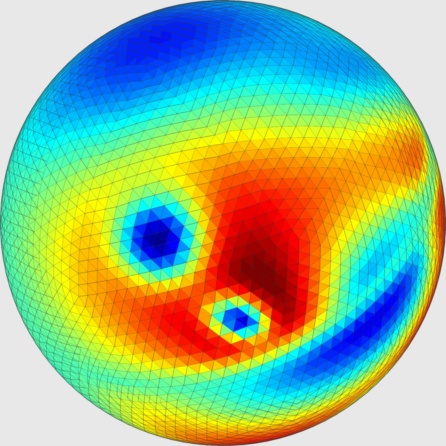
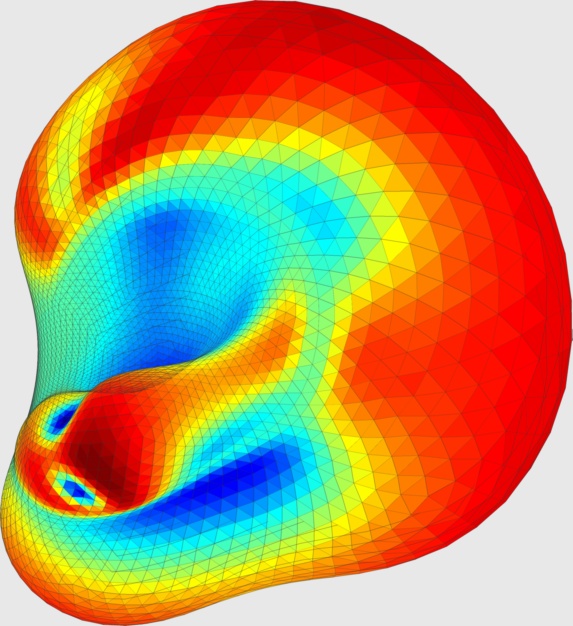
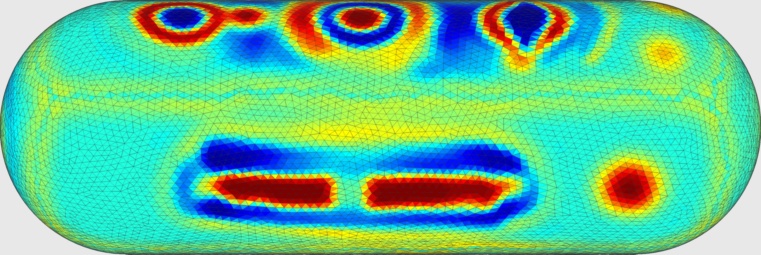
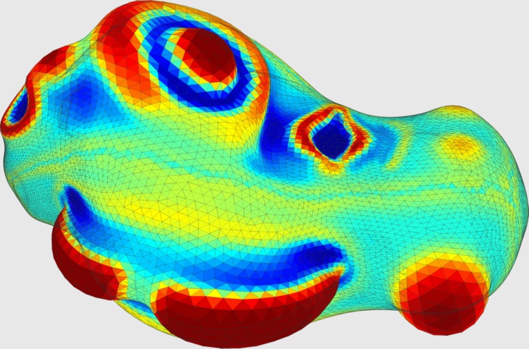
Keenan Crane, Ulrich Pinkall, and Peter Schröder introduced Spin Transformations of Discrete Surfaces at Siggraph 2011. The input to their algorithm is a triangled mesh and a function f that maps each triangle to a real value. The output is a smoothly deformed mesh that has

• bumps with expanded surface area where the function f is positive, and
• dents with contracted surface area where f is negative.

Initially, I started to implement the method according to the derivation in their paper. But then, Keenan made his implementation open-source, so I simply ported his C++ code to Matlab. The examples that are displayed to the side are also taken from Keenans website. The colors of the triangles in the illustrations to the side represent the values of f.

Spin Transformations (Matlab) *

spin.zip

790 kB

* for a demo run spindemo.m in Matlab.

function V=spin(T,V,rho)
% input: T (3xN) and V (3xM) so that
%  trimesh(T',V(1,:),V(2,:),V(3,:)) plots the triangular mesh,
%  rho (1xN) values of conformal scaling
% output: V (3xM) vertices of transformed mesh

nT=size(T,2);
nV=size(V,2);
plc=-3:0;

E=sparse(4*nV,4*nV);
edg=zeros(4,3);
for c1=1:nT
  tri=T(:,c1);
  pnt=V(:,tri);
  A=norm( cross( pnt(:,2)-pnt(:,1) , pnt(:,3)-pnt(:,1) ) )/2;
  a=-1/(4*A);
  b=rho(c1)/6;
  c=jiH([A*rho(c1)*rho(c1)/9 0 0 0]);
  for c2=1:3
    edg(:,c2)=[0;V(:, tri(mod(c2+1,3)+1) )-V(:, tri(mod(c2+0,3)+1) )];
  end  
  ini=[tri(1)*4+plc tri(2)*4+plc tri(3)*4+plc];
  E(ini,ini)=E(ini,ini) + [
    jiH(jiH(a*edg(:,1))*edg(:,1)) + c ...
    jiH(jiH(a*edg(:,1))*edg(:,2) + b*(edg(:,2)-edg(:,1)))+c ...
    jiH(jiH(a*edg(:,1))*edg(:,3) + b*(edg(:,3)-edg(:,1)))+c
    jiH(jiH(a*edg(:,2))*edg(:,1) + b*(edg(:,1)-edg(:,2)))+c ...
    jiH(jiH(a*edg(:,2))*edg(:,2)) + c ...
    jiH(jiH(a*edg(:,2))*edg(:,3) + b*(edg(:,3)-edg(:,2)))+c
    jiH(jiH(a*edg(:,3))*edg(:,1) + b*(edg(:,1)-edg(:,3)))+c ...
    jiH(jiH(a*edg(:,3))*edg(:,2) + b*(edg(:,2)-edg(:,3)))+c ...
    jiH(jiH(a*edg(:,3))*edg(:,3)) + c ];
  if ~mod(c1,500); fprintf('.'); end
end
fprintf('\n')

lam=zeros(4*nV,1);
lam(1:4:end)=1;  
for c1=1:11
  cnv=lam;
  lam=E\lam;
  lam=lam/norm(lam);
end
res=(E*lam)./lam;  
fprintf('mean %e, var %e, delta %e\n',mean(res),var(res),norm(cnv-lam))

L  =sparse(4*nV,4*nV);
ome=zeros(4*nV,1);
for c1=1:nT
  for c2=1:3
    k0=T(mod(c2-1,3)+1,c1);
    k1=T(mod(c2+0,3)+1,c1);
    k2=T(mod(c2+1,3)+1,c1);
    u1=V(:,k1)-V(:,k0);
    u2=V(:,k2)-V(:,k0);
    cta=dot(u1,u2) / norm( cross(u1,u2) );
    h=jiH([cta*0.5 0 0 0]);
    ini=[k1*4+plc  k2*4+plc];
    L(ini,ini)=L(ini,ini)+[ h -h;-h h];
    if k1>k2
      k3=k1; k1=k2; k2=k3; % swap
    end
    lm1=jiH(lam(k1*4+plc));
    lm2=jiH(lam(k2*4+plc));
    edv=jiH([0;V(:,k2)-V(:,k1)]);
    til=lm1'*edv*lm1/3 + lm1'*edv*lm2/6 + lm2'*edv*lm1/6 + lm2'*edv*lm2/3;
    ome(k1*4+plc,1)=ome(k1*4+plc,1)-cta*til(:,1)/2;
    ome(k2*4+plc,1)=ome(k2*4+plc,1)+cta*til(:,1)/2;
  end
  if ~mod(c1,500); fprintf('.'); end
end
fprintf('\n')

ome=reshape(ome,[4 nV]);
ome=ome-repmat(mean(ome,2),[1 nV]);
ome=reshape(ome,[4*nV 1]);
ome=L\ome;
ome=reshape(ome,[4 nV]);
ome=ome-repmat(mean(ome,2),[1 nV]);
nrm=sum(ome.*ome,1);
ome=ome/sqrt(max(nrm));
V=ome(2:end,:);

function h=jiH(pnt)
a=pnt(1); b=pnt(2); c=pnt(3); d=pnt(4);
h=[ a -b -c -d
    b  a -d  c
    c  d  a -b
    d -c  b  a];

Those who make peaceful revolution impossible
will make violent revolution inevitable.
John Fitzgerald Kennedy